PLato said,"Look to the perfection of the heavens for truth," while Aristotle said "look around you at what is, if you would know the truth" To Remember: Eskesthai
In networking, black holes refer to places in the network where incoming traffic is silently discarded (or “dropped”), without informing the source that the data did not reach its intended recipient.
When examining the topology of the network, the black holes themselves are invisible, and can only be detected by monitoring the lost traffic; hence the name.
The most common form of black hole is simply an IP address that specifies a host machine that is not running or an address to which no host has been assigned. Even though TCP/IP provides means of communicating the delivery failure back to the sender via ICMP, traffic destined for such addresses is often just dropped. Note that a dead address will be undetectable only to protocols that are both connectionless and unreliable (e.g., UDP). Connection-oriented or reliable protocols (TCP, RUDP) will either fail to connect to a dead address or will fail to receive expected acknowledgements.
Firewalls and “stealth” ports
Most firewalls can be configured to silently discard packets addressed to forbidden hosts or ports, resulting in small or large “black holes” in the network.
Black hole filtering
Black hole filtering refers specifically to dropping packets at the routing level, usually using a routing protocol to implement the filtering on several routers at once, often dynamically to respond quickly to distributed denial-of-service attacks.
Some firewalls incorrectly discard all ICMP packets, including the ones needed for Path MTU discovery to work correctly. This causes TCP connections from/to/through hosts with a lower MTU to hang.
Black hole e-mail addresses
A black hole e-mail address is an e-mail address which is valid (messages sent to it will not generate errors), but to which all messages sent are automatically deleted, and never stored or seen by humans. These addresses are often used as return addresses for automated e-mails.
At any given moment about 2,000 thunderstorms roll over Earth, producing some 50 flashes of lightning every second. Each lightning burst creates electromagnetic waves that begin to circle around Earth captured between Earth’s surface and a boundary about 60 miles up. Some of the waves – if they have just the right wavelength – combine, increasing in strength, to create a repeating atmospheric heartbeat known as Schumann resonance. This resonance provides a useful tool to analyze Earth’s weather, its electric environment, and to even help determine what types of atoms and molecules exist in Earth’s atmosphere.
The waves created by lightning do not look like the up and down waves of the ocean, but they still oscillate with regions of greater energy and lesser energy. These waves remain trapped inside an atmospheric ceiling created by the lower edge of the “ionosphere” – a part of the atmosphere filled with charged particles, which begins about 60 miles up into the sky. In this case, the sweet spot for resonance requires the wave to be as long (or twice, three times as long, etc) as the circumference of Earth. This is an extremely low frequency wave that can be as low as 8 Hertz (Hz) – some one hundred thousand times lower than the lowest frequency radio waves used to send signals to your AM/FM radio. As this wave flows around Earth, it hits itself again at the perfect spot such that the crests and troughs are aligned. Voila, waves acting in resonance with each other to pump up the original signal.
While they’d been predicted in 1952, Schumann resonances were first measured reliably in the early 1960s. Since then, scientists have discovered that variations in the resonances correspond to changes in the seasons, solar activity, activity in Earth’s magnetic environment, in water aerosols in the atmosphere, and other Earth-bound phenomena. See: Schumann resonance animation
This global electromagnetic resonance phenomenon is named after physicist Winfried Otto Schumann who predicted it mathematically in 1952. Schumann resonances occur because the space between the surface of the Earth and the conductive ionosphere acts as a closed waveguide. The limited dimensions of the Earth cause this waveguide to act as a resonant cavity for electromagnetic waves in the ELF band. The cavity is naturally excited by electric currents in lightning. Schumann resonances are the principal background in the electromagnetic spectrum[1] beginning at 3 Hz and extend to 60 Hz,[2] and appear as distinct peaks at extremely low frequencies (ELF) around 7.86 (fundamental),[3] 14.3, 20.8, 27.3 and 33.8 Hz.[4][5]
In the normal mode descriptions of Schumann resonances, the fundamental mode is a standing wave in the Earth–ionosphere cavity with a wavelength equal to the circumference of the Earth. This lowest-frequency (and highest-intensity) mode of the Schumann resonance occurs at a frequency of approximately 7.86 Hz, but this frequency can vary slightly from a variety of factors, such as solar-induced perturbations to the ionosphere, which comprises the upper wall of the closed cavity[citation needed]. The higher resonance modes are spaced at approximately 6.5 Hz intervals[citation needed], a characteristic attributed to the atmosphere’s spherical geometry. The peaks exhibit a spectral width of approximately 20% on account of the damping of the respective modes in the dissipative cavity. The eighth overtone lies at approximately 59.9 Hz.[citation needed]
Observations of Schumann resonances have been used to track global lightning activity. Owing to the connection between lightning activity and the Earth’s climate it has been suggested that they may also be used to monitor global temperature variations and variations of water vapor in the upper troposphere. It has been speculated that extraterrestrial lightning (on other planets) may also be detected and studied by means of their Schumann resonance signatures. Schumann resonances have been used to study the lower ionosphere on Earth and it has been suggested as one way to explore the lower ionosphere on celestial bodies. Effects on Schumann resonances have been reported following geomagnetic and ionospheric disturbances. More recently, discrete Schumann resonance excitations have been linked to transient luminous events – sprites, elves, jets, and other upper-atmospheric lightning. A new field of interest using Schumann resonances is related to short-term earthquake prediction.
History
The first documented observations of global electromagnetic resonance were made by Nikola Tesla at his Colorado Springs laboratory in 1899. This observation led to certain peculiar conclusions about the electrical properties of the Earth, and which made the basis for his idea for wireless energy transmission.[6]
Tesla researched ways to transmit power and energy wirelessly over long distances (via transverse waves and longitudinal waves). He transmitted extremely low frequencies through the ground as well as between the Earth’s surface and the Kennelly-Heaviside layer. He received patents on wireless transceivers that developed standing waves by this method. Making mathematical calculations based on his experiments, Tesla discovered that the resonant frequency of the Earth was approximately 8 hertz (Hz).[citation needed] In the 1950s, researchers confirmed that the resonant frequency of the Earth’s ionospheric cavity was in this range (later named the Schumann resonance).
The first suggestion that an ionosphere existed, capable of trapping electromagnetic waves, was made by Heaviside and Kennelly in 1902.[7][8] It took another twenty years before Edward Appleton and Barnett in 1925,[9] were able to prove experimentally the existence of the ionosphere.
Although some of the most important mathematical tools for dealing with spherical waveguides were developed by G. N. Watson in 1918,[10] it was Winfried Otto Schumann who first studied the theoretical aspects of the global resonances of the earth–ionosphere waveguide system, known today as the Schumann resonances. In 1952–1954 Schumann, together with H. L. König, attempted to measure the resonant frequencies.[11][12][13][14] However, it was not until measurements made by Balser and Wagner in 1960–1963[15][16][17][18][19] that adequate analysis techniques were available to extract the resonance information from the background noise. Since then there has been an increasing interest in Schumann resonances in a wide variety of fields.
Basic theory
Lightning discharges are considered to be the primary natural source of Schumann resonance excitation; lightning channels behave like huge antennas that radiate electromagnetic energy at frequencies below about 100 kHz.[20] These signals are very weak at large distances from the lightning source, but the Earth–ionosphere waveguide behaves like a resonator at ELF frequencies and amplifies the spectral signals from lightning at the resonance frequencies.[20]
The real Earth–ionosphere waveguide is not a perfect electromagnetic resonant cavity. Losses due to finite ionosphere electrical conductivity lower the propagation speed of electromagnetic signals in the cavity, resulting in a resonance frequency that is lower than would be expected in an ideal case, and the observed peaks are wide. In addition, there are a number of horizontal asymmetries – day-night difference in the height of the ionosphere, latitudinal changes in the Earth magnetic field, sudden ionospheric disturbances, polar cap absorption, etc. that produce other effects in the Schumann resonance power spectra.
Measurements
Today Schumann resonances are recorded at many separate research stations around the world. The sensors used to measure Schumann resonances typically consist of two horizontal magnetic inductive coils for measuring the north-south and east-west components of the magnetic field, and a vertical electric dipole antenna for measuring the vertical component of the electric field. A typical passband of the instruments is 3–100 Hz. The Schumann resonance electric field amplitude (~300 microvolts per meter) is much smaller than the static fair-weather electric field (~150 V/m) in the atmosphere. Similarly, the amplitude of the Schumann resonance magnetic field (~1 picotesla) is many orders of magnitude smaller than the Earth magnetic field (~30–50 microteslas).[21] Specialized receivers and antennas are needed to detect and record Schumann resonances. The electric component is commonly measured with a ball antenna, suggested by Ogawa et al., in 1966,[22] connected to a high-impedance amplifier. The magnetic induction coils typically consist of tens- to hundreds-of-thousands of turns of wire wound around a core of very high magnetic permeability.
Dependence on global lightning activity
From the very beginning of Schumann resonance studies, it was known that they could be used to monitor global lightning activity. At any given time there are about 2000 thunderstorms around the globe.[23] Producing ~50 lightning events per second,[24] these thunderstorms create the background Schumann resonance signal.
Determining the spatial lightning distribution from Schumann resonance records is a complex problem: in order to estimate the lightning intensity from Schumann resonance records it is necessary to account for both the distance to lightning sources as well as the wave propagation between the source and the observer. The common approach is to make a preliminary assumption on the spatial lightning distribution, based on the known properties of lightning climatology. An alternative approach is placing the receiver at the North or South Pole, which remain approximately equidistant from the main thunderstorm centers during the day.[25] One method not requiring preliminary assumptions on the lightning distribution[26] is based on the decomposition of the average background Schumann resonance spectra, utilizing ratios between the average electric and magnetic spectra and between their linear combination. This technique assumes the cavity is spherically symmetric and therefore does not include known cavity asymmetries that are believed to affect the resonance and propagation properties of electromagnetic waves in the system.
Diurnal variations
The best documented and the most debated features of the Schumann resonance phenomenon are the diurnal variations of the background Schumann resonance power spectrum.
A characteristic Schumann resonance diurnal record reflects the properties of both global lightning activity and the state of the Earth–ionosphere cavity between the source region and the observer. The vertical electric field is independent of the direction of the source relative to the observer, and is therefore a measure of global lightning. The diurnal behavior of the vertical electric field shows three distinct maxima, associated with the three “hot spots” of planetary lightning activity: 9 UT (Universal Time) peak, linked to the increased thunderstorm activity from south-east Asia; 14 UT peak associated with the peak in African lightning activity; and the 20 UT peak resulting for the increase in lightning activity in South America. The time and amplitude of the peaks vary throughout the year, reflecting the seasonal changes in lightning activity.
“Chimney” ranking
In general, the African peak is the strongest, reflecting the major contribution of the African “chimney” to the global lightning activity. The ranking of the two other peaks – Asian and American – is the subject of a vigorous dispute among Schumann resonance scientists. Schumann resonance observations made from Europe show a greater contribution from Asia than from South America. This contradicts optical satellite and climatological lightning data that show the South American thunderstorm center stronger than the Asian center.,[24] although observations made from North America indicate the dominant contribution comes from South America. The reason for such disparity remains unclear, but may have something to do with the 60 Hz cycling of electricity used in North America (60 Hz being a mode of Schumann Resonance). Williams and Sátori[27] suggest that in order to obtain “correct” Asia-America chimney ranking, it is necessary to remove the influence of the day/night variations in the ionospheric conductivity (day-night asymmetry influence) from the Schumann resonance records. On the other hand, such “corrected” records presented in the work by Sátori et al.[28] show that even after the removal of the day-night asymmetry influence from Schumann resonance records, the Asian contribution remains greater than American. Similar results were obtained by Pechony et al.[29] who calculated Schumann resonance fields from satellite lightning data. It was assumed that the distribution of lightning in the satellite maps was a good proxy for Schumann excitations sources, even though satellite observations predominantly measure in-cloud lightning rather than the cloud-to-ground lightning that are the primary exciters of the resonances. Both simulations – those neglecting the day-night asymmetry, and those taking this asymmetry into account, showed same Asia-America chimney ranking. As for today, the reason for the “invert” ranking of Asia and America chimneys in Schumann resonance records remains unclear and the subject requires further, targeted research.
Influence of the day-night asymmetry
In the early literature the observed diurnal variations of Schumann resonance power were explained by the variations in the source-receiver (lightning-observer) geometry.[15] It was concluded that no particular systematic variations of the ionosphere (which serves as the upper waveguide boundary) are needed to explain these variations.[30] Subsequent theoretical studies supported the early estimations of the small influence of the ionosphere day-night asymmetry (difference between day-side and night-side ionosphere conductivity) on the observed variations in Schumann resonance field intensities.[31]
The interest in the influence of the day-night asymmetry in the ionosphere conductivity on Schumann resonances gained new strength in the 1990s, after publication of a work by Sentman and Fraser.[32] Sentman and Fraser developed a technique to separate the global and the local contributions to the observed field power variations using records obtained simultaneously at two stations that were widely separated in longitude. They interpreted the diurnal variations observed at each station in terms of a combination of a diurnally varying global excitation modulated by the local ionosphere height. Their work, which combined both observations and energy conservation arguments, convinced many scientists of the importance of the ionospheric day-night asymmetry and inspired numerous experimental studies. However, recently it was shown that results obtained by Sentman and Fraser can be approximately simulated with a uniform model (without taking into account ionosphere day-night variation) and therefore cannot be uniquely interpreted solely in terms of ionosphere height variation.[33]
Schumann resonance amplitude records show significant diurnal and seasonal variations which in general coincide in time with the times of the day-night transition (the terminator). This time-matching seems to support the suggestion of a significant influence of the day-night ionosphere asymmetry on Schumann resonance amplitudes. There are records showing almost clock-like accuracy of the diurnal amplitude changes.[28] On the other hand there are numerous days when Schumann Resonance amplitudes do not increase at sunrise or do not decrease at sunset. There are studies showing that the general behavior of Schumann resonance amplitude records can be recreated from diurnal and seasonal thunderstorm migration, without invoking ionospheric variations.[29][31] Two recent independent theoretical studies have shown that the variations in Schumann resonance power related to the day-night transition are much smaller than those associated with the peaks of the global lightning activity, and therefore the global lightning activity plays a more important role in the variation of the Schumann resonance power.[29][34]
It is generally acknowledged that source-observer effects are the dominant source of the observed diurnal variations, but there remains considerable controversy about the degree to which day-night signatures are present in the data. Part of this controversy stems from the fact that the Schumann resonance parameters extractable from observations provide only a limited amount of information about the coupled lightning source-ionospheric system geometry. The problem of inverting observations to simultaneously infer both the lightning source function and ionospheric structure is therefore extremely underdetermined, leading to the possibility of nonunique interpretations.
The “inverse problem”
One of the interesting problems in Schumann resonances studies is determining the lightning source characteristics (the “inverse problem”). Temporally resolving each individual flash is impossible because the mean rate of excitation by lightning, ~50 lightning events per second globally, mixes up the individual contributions together. However, occasionally there occur extremely large lightning flashes which produce distinctive signatures that stand out from the background signals. Called “Q-bursts”, they are produced by intense lightning strikes that transfer large amounts of charge from clouds to the ground, and often carry high peak current.[22] Q-bursts can exceed the amplitude of the background signal level by a factor of 10 or more, and appear with intervals of ~10 s,[26] which allows to consider them as isolated events and determine the source lightning location. The source location is determined with either multi-station or single-station techniques, and requires assuming a model for the Earth–ionosphere cavity. The multi-station techniques are more accurate, but require more complicated and expensive facilities.
Transient luminous events research
It is now believed that many of the Schumann resonances transients (Q bursts) are related to the transient luminous events (TLEs). In 1995 Boccippio et al.[35] showed that sprites, the most common TLE, are produced by positive cloud-to-ground lightning occurring in the stratiform region of a thunderstorm system, and are accompanied by Q-burst in the Schumann resonances band. Recent observations[35][36] reveal that occurrences of sprites and Q bursts are highly correlated and Schumann resonances data can possibly be used to estimate the global occurrence rate of sprites.[37]
Global temperature
Williams [1992][38] suggested that global temperature may be monitored with the Schumann resonances. The link between Schumann resonance and temperature is lightning flash rate, which increases nonlinearly with temperature.[38] The nonlinearity of the lightning-to-temperature relation provides a natural amplifier of the temperature changes and makes Schumann resonance a sensitive “thermometer”. Moreover, the ice particles that are believed to participate in the electrification processes which result in a lightning discharge[39] have an important role in the radiative feedback effects that influence the atmosphere temperature. Schumann resonances may therefore help us to understand these feedback effects. A strong link between global lightning and global temperature has not been experimentally confirmed as of 2008.
Upper tropospheric water vapor
Tropospheric water vapor is a key element of the Earth’s climate, which has direct effects as a greenhouse gas, as well as indirect effect through interaction with clouds, aerosols and tropospheric chemistry. Upper tropospheric water vapor (UTWV) has a much greater impact on the greenhouse effect than water vapor in the lower atmosphere,[40] but whether this impact is a positive, or a negative feedback is still uncertain.[41] The main challenge in addressing this question is the difficulty in monitoring UTWV globally over long timescales. Continental deep-convective thunderstorms produce most of the lightning discharges on Earth. In addition, they transport large amount of water vapor into the upper troposphere, dominating the variations of global UTWV. Price [2000][42] suggested that changes in the UTWV can be derived from records of Schumann Resonances. According to the effective work made by the Upper Tropospheric Water Vapor (( UTWV )), we should highlight that the percentage of UTWV in normal condition of the Air mass can be meauserd as a minimal quantity, so that its influence can be considered very very low; in fact the higher percentage of it can be only found in the lower Tropspheric layers. But in the case of a high quantity of UTWV in the highest level of Troposphere, due to a warmer air mass of atlantic origins, for istance, the Water vapor, due to the low air temperature ((about minus 60 Degrees )) it turns into ice cristal, becoming clouds as Cirrus or Cirrus Stratus: no Water vapour exists as gas with so low temperature. So, we can say that the affirmation that Water vapor interacts with cloud, can be considered wrong as the clouds both those of low level of ((Atmosphere)) and those of higher levels of it are made of condensed or cristallised Water Vapor.
Schumann resonances on other planets
The existence of Schumann-like resonances is conditioned primarily by two factors: (1) a closed, planetary-sized spherical[dubious– discuss] cavity, consisting of conducting lower and upper boundaries separated by an insulating medium. For the earth the conducting lower boundary is its surface, and the upper boundary is the ionosphere. Other planets may have similar electrical conductivity geometry, so it is speculated that they should possess similar resonant behavior. (2) source of electrical excitation of electromagnetic waves in the ELF range. Within the Solar System there are five candidates for Schumann resonance detection besides the Earth: Venus, Mars, Jupiter, Saturn and its moon Titan.
Modeling Schumann resonances on the planets and moons of the Solar System is complicated by the lack of knowledge of the waveguide parameters. No in situ capability exists today to validate the results, but in the case of Mars there have been terrestrial observations of radio emission spectra that have been associated with Schumann resonances.[43] The reported radio emissions are not of the primary electromagnetic Schumann modes, but rather of secondary modulations of the nonthermal microwave emissions from the planet at approximately the expected Schumann frequencies, and have not been independently confirmed to be associated with lightning activity on Mars. There is the possibility that future lander missions could carry in situ instrumentation to perform the necessary measurements. Theoretical studies are primarily directed to parameterizing the problem for future planetary explorers.
The strongest evidence for lightning on Venus comes from the impulsive electromagnetic waves detected by Venera 11 and 12 landers. Theoretical calculations of the Schumann resonances at Venus were reported by Nickolaenko and Rabinowicz [1982][44] and Pechony and Price [2004].[45] Both studies yielded very close results, indicating that Schumann resonances should be easily detectable on that planet given a lightning source of excitation and a suitably located sensor.
On Mars detection of lightning activity has been reported by Ruf et al. [2009].[43] The evidence is indirect and in the form of modulations of the nonthermal microwave spectrum at approximately the expected Schumann resonance frequencies. It has not been independently confirmed that these are associated with electrical discharges on Mars. In the event confirmation is made by direct, in situ observations, it would verify the suggestion of the possibility of charge separation and lightning strokes in the Martian dust storms made by Eden and Vonnegut [1973][46] and Renno et al. [2003].[47] Martian global resonances were modeled by Sukhorukov [1991],[48] Pechony and Price [2004][45] and Molina-Cuberos et al. [2006].[49] The results of the three studies are somewhat different, but it seems that at least the first two Schumann resonance modes should be detectable. Evidence of the first three Schumann resonance modes is present in the spectra of radio emission from the lightning detected in Martian dust storms.[43]
It was long ago suggested that lightning discharges may occur on Titan,[50] but recent data from Cassini–Huygens seems to indicate that there is no lightning activity on this largest satellite of Saturn. Due to the recent interest in Titan, associated with the Cassini–Huygens mission, its ionosphere is perhaps the most thoroughly modeled today. Schumann resonances on Titan have received more attention than on any other celestial body, in works by Besser et al. [2002],[51] Morente et al. [2003],[52] Molina-Cuberos et al. [2004],[53] Nickolaenko et al. [2003][54] and Pechony and Price [2004].[45] It appears that only the first Schumann resonance mode might be detectable on Titan.
Jupiter is the only planet where lightning activity has been optically detected. Existence of lightning activity on that planet was predicted by Bar-Nun [1975][55] and it is now supported by data from Galileo, Voyagers 1 and 2, Pioneers 10 and 11 and Cassini. Saturn is also expected to have intensive lightning activity, but the three visiting spacecrafts – Pioneer 11 in 1979, Voyager 1 in 1980 and Voyager 2 in 1981, failed to provide any convincing evidence from optical observations. The strong storm monitored on Saturn by the Cassini spacecraft produced no visible lightning flashes, although electromagnetic sensors aboard the spacecraft detected signatures that are characteristic of lightning. Little is known about the electrical parameters of Jupiter and Saturn interior. Even the question of what should serve as the lower waveguide boundary is a non-trivial one in case of the gaseous planets. There seem to be no works dedicated to Schumann resonances on Saturn. To date there has been only one attempt to model Schumann resonances on Jupiter.[56] Here, the electrical conductivity profile within the gaseous atmosphere of Jupiter was calculated using methods similar to those used to model stellar interiors, and it was pointed out that the same methods could be easily extended to the other gas giants Saturn, Uranus and Neptune. Given the intense lightning activity at Jupiter, the Schumann resonances should be easily detectable with a sensor suitably positioned within the planetary-ionospheric cavity.
Speculation about Schumann resonance effects in non-geophysics domains
Interest in Schumann resonances extends beyond the domain of geophysics where it initially began, to the fields of bioenergetics[57] and acupuncture.[57] Critics[who?] claim that the studies that support these applications are inconclusive and that further studies are needed.
A small study in Japan found that blood pressure was lowered by the Schumann resonance, with the effects on human health needing to be investigated further.[58]
^The electrical nature of storms By D. R. MacGorman, W. D. Rust, W. David Rust. Page 114.
^Handbook of atmospheric electrodynamics, Volume 1 By Hans Volland. Page 277.
^A to Z of scientists in weather and climate By Don Rittner. Page 197.
^The electrical nature of storms By D. R. MacGorman, W. D. Rust, W. David Rust. Page 114.
^Recent advances in multidisciplinary applied physics By A. Méndez-Vilas. Page 65.
^N. Tesla (1905). “The Transmission of Electrical Energy Without Wires As A Means Of Furthering World Peace”. Electrical World and EngineerJanuary 7: 21–24.
^A.E. Kennelly (1902). “On the elevation of the electrically-conducting strata of the earth’s atmosphere”. Electrical world and engineer32: 473–473.
^Appleton, E. V. , M. A. F. Barnett (1925). “On Some Direct Evidence for Downward Atmospheric Reflection of Electric Rays”. Proceedings of the Royal Society of London. Series A, Containing Papers of a Mathematical and Physical Character109 (752): 621–641. Bibcode1925RSPSA.109..621A. DOI:10.1098/rspa.1925.0149.
^Watson, G.N. (1918). “The diffraction of electric waves by the Earth”. Proc. Roy. Soc. (London)Ser.A 95: 83–99.
^ abSchumann W. O. (1952). “Über die strahlungslosen Eigenschwingungen einer leitenden Kugel, die von einer Luftschicht und einer Ionosphärenhülle umgeben ist”. Zeitschrift und Naturfirschung7a: 149–154. Bibcode1952ZNatA…7..149S.
^Schumann W. O. (1952). “Über die Dämpfung der elektromagnetischen Eigenschwingnugen des Systems Erde – Luft – Ionosphäre”. Zeitschrift und Naturfirschung7a: 250–252. Bibcode1952ZNatA…7..250S.
^Schumann W. O. (1952). “Über die Ausbreitung sehr Langer elektriseher Wellen um die Signale des Blitzes”. Nuovo Cimento9 (12): 1116–1138. DOI:10.1007/BF02782924.
^Balser M. and C. Wagner (1962). “Diurnal power variations of the Earth–ionosphere cavity modes and their relationship to worldwide thunderstorm activity”. J.G.R67 (2): 619–625. Bibcode1962JGR….67..619B. DOI:10.1029/JZ067i002p00619.
^Balser M. and C. Wagner (1963). “Effect of a high-altitude nuclear detonation on the Earth–ionosphere cavity”. J.G.R68: 4115–4118.
^ abVolland, H. (1984). Atmospheric Electrodynamics. Springer-Verlag, Berlin.
^Price, C., O. Pechony, E. Greenberg (2006). “Schumann resonances in lightning research”. Journal of Lightning Research1: 1– 15.
^ abOgawa, T., Y. Tanka, T. Miura, and M. Yasuhara (1966). “Observations of natural ELF electromagnetic noises by using the ball antennas”. J. Geomagn. Geoelectr18: 443– 454.
^Heckman S. J., E. Williams, (1998). “Total global lightning inferred from Schumann resonance measurements”. J. G. R.103(D24): 31775–31779. Bibcode1998JGR…10331775H. DOI:10.1029/98JD02648.
^ abChristian H. J., R.J. Blakeslee, D.J. Boccippio, W.L. Boeck, D.E. Buechler, K.T. Driscoll, S.J. Goodman, J.M. Hall, W.J. Koshak, D.M. Mach, M.F. Stewart, (2003). “Global frequency and distribution of lightning as observed from space by the Optical Transient Detector”. J. G. R.108(D1): 4005. Bibcode2003JGRD..108.4005C. DOI:10.1029/2002JD002347.
^ abShvets A.V. (2001). “A technique for reconstruction of global lightning distance profile from background Schumann resonance signal”. J.a.s.t.p.63: 1061–1074.
^Williams E. R., G. Sátori (2004). “Lightning, thermodynamic and hydrological comparison of the two tropical continental chimneys”. J.a.s.t.p.66: 1213–1231.
^ abSátori G., M. Neska, E. Williams, J. Szendrői (2007). “Signatures of the non-uniform Earth–ionosphere cavity in high time-resolution Schumann resonance records”. Radio Sciencein print.
^ abcPechony, O., C. Price, A.P. Nickolaenko (2007). “Relative importance of the day-night asymmetry in Schumann resonance amplitude records”. Radio Sciencein print.
^ abNickolaenko A. P. and M. Hayakawa (2002). Resonances in the Earth–ionosphere cavity. Kluwer Academic Publishers, Dordrecht-Boston-London.
^Sentman, D.D., B. J. Fraser (1991). “Simultaneous observations of Schumann Resonances in California and Australia – Evidence for intensity modulation by the local height of the D region”. Journal of geophysical research96 (9): 15973–15984. Bibcode1991JGR….9615973S. DOI:10.1029/91JA01085.
^Yang H., V. P. Pasko (2007). “Three-dimensional finite difference time domain modeling of the diurnal and seasonal variations in Schumann resonance parameters”. Radio Science41 (2): RS2S14. Bibcode2006RaSc…41.2S14Y. DOI:10.1029/2005RS003402.
^Price, C., E. Greenberg, Y. Yair, G. Sátori, J. Bór, H. Fukunishi, M. Sato, P. Israelevich, M. Moalem, A. Devir, Z. Levin, J.H. Joseph, I. Mayo, B. Ziv, A. Sternlieb (2004). “Ground-based detection of TLE-producing intense lightning during the MEIDEX mission on board the Space Shuttle Columbia”. G.R.L.31.
^Hansen, J., A. Lacis, D. Rind, G. Russel, P. Stone, I. Fung, R. Ruedy, J., Lerner (1984). “Climate sensitivity: Analysis of feedback mechanisms”. Climate Processes and Climate Sensitivity, J.,E. Hansen and T. Takahashi, eds.. AGU Geophys. Monograph29: 130–163.
^Price, C. (2000). “Evidence for a link between global lightning activity and upper tropospheric water vapor”. Letters to Nature406 (6793): 290–293. DOI:10.1038/35018543. PMID10917527.
^ abcRuf, C., N. O. Renno, J. F. Kok, E. Bandelier, M. J. Sander, S. Gross, L. Skjerve, and B. Cantor (2009). “Emission of Non-thermal Microwave Radiation by a Martian Dust Storm”. Geophys. Res. Lett.36 (13): L13202. Bibcode2009GeoRL..3613202R. DOI:10.1029/2009GL038715.
^Nickolaenko A. P., L. M. Rabinowicz (1982). “On the possibility of existence of global electromagnetic resonances on the planets of Solar system”. Space Res.20: 82–89.
^ abcPechony, O., C. Price (2004). “Schumann resonance parameters calculated with a partially uniform knee model on Earth, Venus, Mars, and Titan”. Radio Sci.39 (5): RS5007. Bibcode2004RaSc…39.5007P. DOI:10.1029/2004RS003056.
^Renno N. O., A. Wong, S. K. Atreya, I. de Pater, M. Roos-Serote (2003). “Electrical discharges and broadband radio emission by Martian dust devils and dust storms”. G. R. L.30 (22): 2140. Bibcode2003GeoRL..30vPLA1R. DOI:10.1029/2003GL017879.
^Molina-Cuberos G. J., J. A. Morente, B. P. Besser, J. Porti, H. Lichtenegger, K. Schwingenschuh, A. Salinas, J. Margineda (2006). “Schumann resonances as a tool to study the lower ionosphere of Mars”. Radio Science41: RS1003. Bibcode2006RaSc…41.1003M. DOI:10.1029/2004RS003187.
^Lammer H., T. Tokano, G. Fischer, W. Stumptner, G. J. Molina-Cuberos, K. Schwingenschuh, H. O. Rucher (2001). “Lightning activity of Titan: can Cassiny/Huygens detect it?”. Planet. Space Sci.49 (6): 561–574. Bibcode2001P&SS…49..561L. DOI:10.1016/S0032-0633(00)00171-9.
^Besser, B. P., K. Schwingenschuh, I. Jernej, H. U. Eichelberger, H. I. M. Lichtenegger, M. Fulchignoni, G. J. Molina-Cuberos, J. A. Morente, J. A. Porti, A. Salinas (2002). “Schumann resonances as indicators for lighting on Titan”. Proceedings of the Second European Workshop on Exo/Astrobiology, Graz, Australia, 16–19 September.
^Morente J. A., Molina-Cuberos G. J., Porti J. A., K. Schwingenschuh, B. P. Besser (2003). “A study of the propagation of electromagnetic waves in Titan’s atmosphere with the TLM numerical method”. Icarus162 (2): 374–384. Bibcode2003Icar..162..374M. DOI:10.1016/S0019-1035(03)00025-3.
^Molina-Cuberos G. J., J. Porti, B. P. Besser, J. A. Morente, J. Margineda, H. I. M. Lichtenegger, A. Salinas, K. Schwingenschuh, H. U. Eichelberger (2004). “Shumann resonances and electromagnetic transparence in the atmosphere of Titan”. Advances in Space Research33 (12): 2309–2313. Bibcode2004AdSpR..33.2309M. DOI:10.1016/S0273-1177(03)00465-4.
The data revealed that even the most complex, abstract emotions—those that require maturity, reflection, and world knowledge to appreciate—do involve our most advanced brain networks. However, they seem to get their punch—their motivational push—from activating basic biological regulatory structures in the most primitive parts of the brain, those responsible for monitoring functions like heart rate and breathing. In turn, the basic bodily changes induced during even the most complex emotions—e.g., our racing heart or clenched gut—are “felt” by sensory brain networks. When we talk of having a gut feeling that some action is right or wrong, we are not just speaking metaphorically.
So, I’m saying the mirror neuron system underlies the interface allowing you to rethink about issues like consciousness,representation of self,what separates you from other human beings,what allows you to empathize with other human beings,and also even things like the emergence of culture and civilization,which is unique to human beings. See: VS Ramachandran: The neurons that shaped civilization
How important is the environment in that we might see the development of the conditions of “specific types of neurons” when the color can dictate the type of neuron developed? Can we say that the color(emotion) is an emotive state that we might indeed create in the type of consciousness with which we meet the world. A consciousness that that sets the trains of thought given the reality of our own perceptions. Or, perpetuated thought processes unravelled in a world of our own illusions?
In a nutshell, what Karim showed was that each time a memory is used, it has to be restored as a new memory in order to be accessible later. The old memory is either not there or is inaccessible. In short, your memory about something is only as good as your last memory about it. Joseph LeDoux
Psychology professor Karim Nader is helping sufferers of post-traumatic stress disorder lessen debilitating symptoms—and in some cases, regain a normal life.Owen Egan See also: The Trauma TamerSee Also: Brain Storming
IC: Why is this research so important?
Karim Nader: There are a lot of implications. All psychopathological disorders, such as PTSD, epilepsy, obsessive compulsive disorders, or addiction—all these things have to do with your brain getting rewired in a way that is malfunctioning. Theoretically, we may be able to treat a lot of these psychopathologies. If you could block the re-storage of the circuit that causes the obsessive compulsion, then you might be able to reset a person to a level where they aren’t so obsessive. Or perhaps you can reset the circuit that has undergone epilepsy repeatedly so that you can increase the threshold for seizures. And there is some killer data showing that it’s possible to block the reconsolidation of drug cravings.
The other reason why I think it is so striking is that it is so contrary to what has been the accepted view of memory for so long in the mainstream. My research caused everybody in the field to stop, turn around and go, “Whoa, where’d that come from?” Nobody’s really working on this issue, and the only reason I came up with this is because I wasn’t trained in memory. [Nader was originally researching fear.] It really caused a fundamental reconceptualization of a very basic and dogmatic field in neuroscience, which is very exciting. It is the first time in 100 years that people are starting to come up with new models of memory at the physiological level.
Part of the understanding for me is that in creating this environment for neural development the retention of memory has to have some emotive basis which arises from the ancient part of our brain in that it is associated with the heart response.
Here’s an analogy to understand this: imagine that our universe is a two-dimensional pool table, which you look down on from the third spatial dimension. When the billiard balls collide on the table, they scatter into new trajectories across the surface. But we also hear the click of sound as they impact: that’s collision energy being radiated into a third dimension above and beyond the surface. In this picture, the billiard balls are like protons and neutrons, and the sound wave behaves like the graviton. See:The Sound Of Billiard Balls
While these physiological processes are going on in our bodies the chemical responses of emotion trigger manifestations in the world outside of our bodies. Let us say consciousness exists “at the periphery of our bodies.” What measure then to assess the realization that such manifestations internally are in the control of our manipulations of living experience? Are we then not caught in the throes of and are we not machine like to think such associations could have ever been produced in a robot like being manufactured?
Of course this is a fictional representation above of what may resound within and according to the experiences we may have? The question is then how are memories retained? How do memories transmit through out our endocrinology system the nature of our experiences so that we see consciousness as a form of the expression through which we color our world?
It was designed by the RobotCub Consortium, of several European universities and is now supported by other projects such as ITALK.[1] The robot is open-source, with the hardware design, software and documentation all released under the GPL license. The name is a partial acronym, cub standing for Cognitive Universal Body.[2] Initial funding for the project was €8.5 million from Unit E5 – Cognitive Systems and Robotics – of the European Commission‘s Seventh Framework Programme, and this ran for six years from 1 September 2004 until 1 September 2010.[2]
The motivation behind the strongly humanoid design is the embodied cognition hypothesis, that human-like manipulation plays a vital role in the development of human cognition. A baby learns many cognitive skills by interacting with its environment and other humans using its limbs and senses, and consequently its internal model of the world is largely determined by the form of the human body. The robot was designed to test this hypothesis by allowing cognitive learning scenarios to be acted out by an accurate reproduction of the perceptual system and articulation of a small child so that it could interact with the world in the same way that such a child does.[3]
In philosophy, the embodied mind thesis holds that the nature of the human mind is largely determined by the form of the human body. Philosophers, psychologists, cognitive scientists and artificial intelligence researchers who study embodied cognition and the embodied mind argue that all aspects of cognition are shaped by aspects of the body. The aspects of cognition include high level mental constructs (such as concepts and categories) and human performance on various cognitive tasks (such as reasoning or judgement). The aspects of the body include the motor system, the perceptual system, the body’s interactions with the environment (situatedness) and the ontological assumptions about the world that are built into the body and the brain.
Embodied cognition is a topic of research in social and cognitive psychology, covering issues such as social interaction and decision-making.[2] Embodied cognition reflects the argument that the motor system influences our cognition, just as the mind influences bodily actions. For example, when participants hold a pencil in their teeth engaging the muscles of a smile, they comprehend pleasant sentences faster than unpleasant ones.[3] And it works in reverse: holding a pencil in their teeth to engage the muscles of a frown increases the time it takes to comprehend pleasant sentences.[3]
The mind-body problemis a philosophical problem arising in the fields of metaphysics and philosophy of mind.[2] The problem arises because mental phenomena arguably differ, qualitatively or substantially, from the physical body on which they apparently depend. There are a few major theories on the resolution of the problem. Dualism is the theory that the mind and body are two distinct substances,[2] and monism is the theory that they are, in reality, just one substance. Monist materialists (also called physicalists) take the view that they are both matter, and monist idealists take the view that they are both in the mind. Neutral monists take the view that both are reducible to a third, neutral substance.
The problem was identified by René Descartes in the sense known by the modern Western world, although the issue was also addressed by pre-Aristotelian philosophers,[3] in Avicennian philosophy,[4] and in earlier Asian traditions.
A dualist view of reality may lead one to consider the corporeal as little valued[3] and trivial. The rejection of the mind–body dichotomy is found in French Structuralism, and is a position that generally characterized post-war French philosophy.[5] The absence of an empirically identifiable meeting point between the non-physical mind and its physical extension has proven problematic to dualism and many modern philosophers of mind maintain that the mind is not something separate from the body.[6] These approaches have been particularly influential in the sciences, particularly in the fields of sociobiology, computer science, evolutionary psychology and the various neurosciences.[7][8][9][10]
This video takes SDO images and applies additional processing to enhance the structures visible. While there is no scientific value to this processing, it does result in a beautiful, new way of looking at the sun. The original frames are in the 171 Angstrom wavelength of extreme ultraviolet. This wavelength shows plasma in the solar atmosphere, called the corona, that is around 600,000 Kelvin. The loops represent plasma held in place by magnetic fields. They are concentrated in “active regions” where the magnetic fields are the strongest. These active regions usually appear in visible light as sunspots. The events in this video represent 24 hours of activity on September 25, 2011.
Broadband research is a McGill area of expertise. Meet researchers such as David Plant, Tho Le-Ngoc, and Mark Coates who are on the cutting edge of machine to machine communication, high-speed internet technologies, and wireless communications.
The terms are not quite synonymous: “super-Turing computation” usually implies that the proposed model is supposed to be physically realizable, while “hypercomputation” does not.
Technical arguments against the physical realizability of hypercomputations have been presented.
A computational model going beyond Turing machines was introduced by Alan Turing in his 1938 PhD dissertation Systems of Logic Based on Ordinals.[2] This paper investigated mathematical systems in which an oracle was available, which could compute a single arbitrary (non-recursive) function from naturals to naturals. He used this device to prove that even in those more powerful systems, undecidability is still present. Turing’s oracle machines are strictly mathematical abstractions, and are not physically realizable.[3]
Hypercomputation and the Church–Turing thesis
The Church–Turing thesis states that any function that is algorithmically computable can be computed by a Turing machine. Hypercomputers compute functions that a Turing machine cannot, hence, not computable in the Church-Turing sense. An example of a problem a Turing machine cannot solve is the halting problem. A Turing machine cannot decide if an arbitrary program halts or runs forever. Some proposed hypercomputers can simulate the program for an infinite number of steps and tell the user whether or not the program halted.
Hypercomputer proposals
A Turing machine that can complete infinitely many steps. Simply being able to run for an unbounded number of steps does not suffice. One mathematical model is the Zeno machine (inspired by Zeno’s paradox). The Zeno machine performs its first computation step in (say) 1 minute, the second step in ½ minute, the third step in ¼ minute, etc. By summing 1+½+¼+… (a geometric series) we see that the machine performs infinitely many steps in a total of 2 minutes. However, some[who?] people claim that, following the reasoning from Zeno’s paradox, Zeno machines are not just physically impossible, but logically impossible.[4]
Turing’s original oracle machines, defined by Turing in 1939.
In mid 1960s, E Mark Gold and Hilary Putnam independently proposed models of inductive inference (the “limiting recursive functionals”[5] and “trial-and-error predicates”,[6] respectively). These models enable some nonrecursive sets of numbers or languages (including all recursively enumerable sets of languages) to be “learned in the limit”; whereas, by definition, only recursive sets of numbers or languages could be identified by a Turing machine. While the machine will stabilize to the correct answer on any learnable set in some finite time, it can only identify it as correct if it is recursive; otherwise, the correctness is established only by running the machine forever and noting that it never revises its answer. Putnam identified this new interpretation as the class of “empirical” predicates, stating: “if we always ‘posit’ that the most recently generated answer is correct, we will make a finite number of mistakes, but we will eventually get the correct answer. (Note, however, that even if we have gotten to the correct answer (the end of the finite sequence) we are never sure that we have the correct answer.)”[6]L. K. Schubert‘s 1974 paper “Iterated Limiting Recursion and the Program Minimization Problem” [7] studied the effects of iterating the limiting procedure; this allows any arithmetic predicate to be computed. Schubert wrote, “Intuitively, iterated limiting identification might be regarded as higher-order inductive inference performed collectively by an ever-growing community of lower order inductive inference machines.”
A real computer (a sort of idealized analog computer) can perform hypercomputation[8] if physics admits general real variables (not just computable reals), and these are in some way “harnessable” for computation. This might require quite bizarre laws of physics (for example, a measurable physical constant with an oracular value, such as Chaitin’s constant), and would at minimum require the ability to measure a real-valued physical value to arbitrary precision despite thermal noise and quantum effects.
A proposed technique known as fair nondeterminism or unbounded nondeterminism may allow the computation of noncomputable functions.[9] There is dispute in the literature over whether this technique is coherent, and whether it actually allows noncomputable functions to be “computed”.
It seems natural that the possibility of time travel (existence of closed timelike curves (CTCs)) makes hypercomputation possible by itself. However, this is not so since a CTC does not provide (by itself) the unbounded amount of storage that an infinite computation would require. Nevertheless, there are spacetimes in which the CTC region can be used for relativistic hypercomputation.[10] Access to a CTC may allow the rapid solution to PSPACE-complete problems, a complexity class which while Turing-decidable is generally considered computationally intractable.[11][12]
In 1994, Hava Siegelmann proved that her new (1991) computational model, the Artificial Recurrent Neural Network (ARNN), could perform hypercomputation (using infinite precision real weights for the synapses). It is based on evolving an artificial neural network through a discrete, infinite succession of states.[17]
The infinite time Turing machine is a generalization of the Zeno machine, that can perform infinitely long computations whose steps are enumerated by potentially transfinite ordinal numbers. It models an otherwise-ordinary Turing machine for which non-halting computations are completed by entering a special state reserved for reaching a limit ordinal and to which the results of the preceding infinite computation are available.[18]
Jan van Leeuwen and Jiří Wiedermann wrote a 2000 paper[19] suggesting that the Internet should be modeled as a nonuniform computing system equipped with an advice function representing the ability of computers to be upgraded.
A symbol sequence is computable in the limit if there is a finite, possibly non-halting program on a universal Turing machine that incrementally outputs every symbol of the sequence. This includes the dyadic expansion of π and of every other computable real, but still excludes all noncomputable reals. Traditional Turing machines cannot edit their previous outputs; generalized Turing machines, as defined by Jürgen Schmidhuber, can. He defines the constructively describable symbol sequences as those that have a finite, non-halting program running on a generalized Turing machine, such that any output symbol eventually converges, that is, it does not change any more after some finite initial time interval. Due to limitations first exhibited by Kurt Gödel (1931), it may be impossible to predict the convergence time itself by a halting program, otherwise the halting problem could be solved. Schmidhuber ([20][21]) uses this approach to define the set of formally describable or constructively computable universes or constructive theories of everything. Generalized Turing machines can solve the halting problem by evaluating a Specker sequence.
In 1970, E.S. Santos defined a class of fuzzy logic-based “fuzzy algorithms” and “fuzzy Turing machines”.[24] Subsequently, L. Biacino and G. Gerla showed that such a definition would allow the computation of nonrecursive languages; they suggested an alternative set of definitions without this difficulty.[25] Jiří Wiedermann analyzed the capabilities of Santos’ original proposal in 2004.[26]
Dmytro Taranovsky has proposed a finitistic model of traditionally non-finitistic branches of analysis, built around a Turing machine equipped with a rapidly increasing function as its oracle. By this and more complicated models he was able to give an interpretation of second-order arithmetic.[27]
Analysis of capabilities
Many hypercomputation proposals amount to alternative ways to read an oracle or advice function embedded into an otherwise classical machine. Others allow access to some higher level of the arithmetic hierarchy. For example, supertasking Turing machines, under the usual assumptions, would be able to compute any predicate in the truth-table degree containing or . Limiting-recursion, by contrast, can compute any predicate or function in the corresponding Turing degree, which is known to be . Gold further showed that limiting partial recursion would allow the computation of precisely the predicates.
neural networks based on real numbers (Hava Siegelmann)
Criticism
Martin Davis, in his writings on hypercomputation [39][40] refers to this subject as “a myth” and offers counter-arguments to the physical realizability of hypercomputation. As for its theory, he argues against the claims that this is a new field founded in 1990s. This point of view relies on the history of computability theory (degrees of unsolvability, computability over functions, real numbers and ordinals), as also mentioned above. Andrew Hodges wrote a critical commentary[41] on Copeland and Proudfoot’s article[1].
^Alan Turing, 1939, Systems of Logic Based on Ordinals Proceedings London Mathematical Society Volumes 2–45, Issue 1, pp. 161–228.[1]
^“Let us suppose that we are supplied with some unspecified means of solving number-theoretic problems; a kind of oracle as it were. We shall not go any further into the nature of this oracle apart from saying that it cannot be a machine” (Undecidable p. 167, a reprint of Turing’s paper Systems of Logic Based On Ordinals)
^ abcHilary Putnam (1965). “Trial and Error Predicates and the Solution to a Problem of Mostowksi”. Journal of Symbolic Logic30 (1): 49–57. doi:10.2307/2270581. JSTOR2270581.
^Arnold Schönhage, “On the power of random access machines”, in Proc. Intl. Colloquium on Automata, Languages, and Programming (ICALP), pages 520-529, 1979. Source of citation: Scott Aaronson, “NP-complete Problems and Physical Reality”[2] p. 12
^Edith Spaan, Leen Torenvliet and Peter van Emde Boas (1989). “Nondeterminism, Fairness and a Fundamental Analogy”. EATCS bulletin37: 186–193.
^Hajnal Andréka, István Németi and Gergely Székely, Closed Timelike Curves in Relativistic Computation, 2011.[3]
^Todd A. Brun, Computers with closed timelike curves can solve hard problems, Found.Phys.Lett. 16 (2003) 245-253.[4]
^S. Aaronson and J. Watrous. Closed Timelike Curves Make Quantum and Classical Computing Equivalent [5]
^Hogarth, M., 1992, ‘Does General Relativity Allow an Observer to View an Eternity in a Finite Time?’, Foundations of Physics Letters, 5, 173–181.
^István Neméti; Hajnal Andréka (2006). “Can General Relativistic Computers Break the Turing Barrier?”. Logical Approaches to Computational Barriers, Second Conference on Computability in Europe, CiE 2006, Swansea, UK, June 30-July 5, 2006. Proceedings. Lecture Notes in Computer Science. 3988. Springer. doi:10.1007/11780342.
^ abJan van Leeuwen; Jiří Wiedermann (September 2000). “On Algorithms and Interaction”. MFCS ’00: Proceedings of the 25th International Symposium on Mathematical Foundations of Computer Science. Springer-Verlag.
^Jürgen Schmidhuber (2000). “Algorithmic Theories of Everything”. Sections in: Hierarchies of generalized Kolmogorov complexities and nonenumerable universal measures computable in the limit. International Journal of Foundations of Computer Science ():587-612 (). Section 6 in: the Speed Prior: A New Simplicity Measure Yielding Near-Optimal Computable Predictions. in J. Kivinen and R. H. Sloan, editors, Proceedings of the 15th Annual Conference on Computational Learning Theory (COLT ), Sydney, Australia, Lecture Notes in Artificial Intelligence, pages 216–228. Springer, .13 (4): 1–5. arXiv:quant-ph/0011122.
^Davis, Martin, Why there is no such discipline as hypercomputation, Applied Mathematics and Computation, Volume 178, Issue 1, 1 July 2006, Pages 4–7, Special Issue on Hypercomputation
^Davis, Martin (2004). “The Myth of Hypercomputation”. Alan Turing: Life and Legacy of a Great Thinker. Springer.
L. Blum, F. Cucker, M. Shub, S. Smale, Complexity and Real Computation, Springer-Verlag 1997. General development of complexity theory for abstract machines that compute on real numbers instead of bits.
Cooper, S. B.; Odifreddi, P. (2003). “Incomputability in Nature”. In S. B. Cooper and S. S. Goncharov. Computability and Models: Perspectives East and West. Plenum Publishers, New York, Boston, Dordrecht, London, Moscow. pp. 137–160.
Copeland, J. (2002) Hypercomputation, Minds and machines, v. 12, pp. 461–502
In physics and cosmology, digital physics is a collection of theoretical perspectives based on the premise that the universe is, at heart, describable by information, and is therefore computable. Therefore, the universe can be conceived as either the output of a computer program or as a vast, digital computation device (or, at least, mathematically isomorphic to such a device).
Digital physics is grounded in one or more of the following hypotheses; listed in order of increasing strength. The universe, or reality:
is essentially informational (although not every informational ontology needs to be digital);
Digital physics suggests that there exists, at least in principle, a program for a universal computer which computes the evolution of the universe. The computer could be, for example, a huge cellular automaton (Zuse 1967[9]), or a universal Turing machine, as suggested by Schmidhuber (1997), who pointed out that there exists a very short program that can compute all possible computable universes in an asymptotically optimal way.
Some try to identify single physical particles with simple bits. For example, if one particle, such as an electron, is switching from one quantum state to another, it may be the same as if a bit is changed from one value (0, say) to the other (1). A single bit suffices to describe a single quantum switch of a given particle. As the universe appears to be composed of elementary particles whose behavior can be completely described by the quantum switches they undergo, that implies that the universe as a whole can be described by bits. Every state is information, and every change of state is a change in information (requiring the manipulation of one or more bits). Setting aside dark matter and dark energy, which are poorly understood at present, the known universe consists of about 1080protons and the same number of electrons. Hence, the universe could be simulated by a computer capable of storing and manipulating about 1090 bits. If such a simulation is indeed the case, then hypercomputation would be impossible.
Loop quantum gravity could lend support to digital physics, in that it assumes space-time is quantized. Paola Zizzi has formulated a realization of this concept in what has come to be called “computational loop quantum gravity”, or CLQG.[10][11] Other theories that combine aspects of digital physics with loop quantum gravity are those of Marzuoli and Rasetti[12][13] and Girelli and Livine.[14]
Weizsäcker’s ur-alternatives
Physicist Carl Friedrich von Weizsäcker‘s theory of ur-alternatives (archetypal objects), first publicized in his book The Unity of Nature (1980),[15] further developed through the 1990s,[16][17] is a kind of digital physics as it axiomatically constructs quantum physics from the distinction between empirically observable, binary alternatives. Weizsäcker used his theory to derive the 3-dimensionality of space and to estimate the entropy of a proton falling into a black hole.
Pancomputationalism or the computational universe theory
Pancomputationalism (also known as pan-computationalism, naturalist computationalism) is a view that the universe is a huge computational machine, or rather a network of computational processes which, following fundamental physical laws, computes (dynamically develops) its own next state from the current one.[18] A computational universe is proposed by Jürgen Schmidhuber in a paper based on Konrad Zuse’s assumption (1967) that the history of the universe is computable. He pointed out that the simplest explanation of the universe would be a very simple Turing machine programmed to systematically execute all possible programs computing all possible histories for all types of computable physical laws. He also pointed out that there is an optimally efficient way of computing all computable universes based on Leonid Levin‘s universal search algorithm (1973). In 2000 he expanded this work by combining Ray Solomonoff’s theory of inductive inference with the assumption that quickly computable universes are more likely than others. This work on digital physics also led to limit-computable generalizations of algorithmic information or Kolmogorov complexity and the concept of Super Omegas, which are limit-computable numbers that are even more random (in a certain sense) than Gregory Chaitin‘s number of wisdom Omega.
Wheeler’s “it from bit”
Following Jaynes and Weizsäcker, the physicist John Archibald Wheeler wrote the following:
[…] it is not unreasonable to imagine that information sits at the core of physics, just as it sits at the core of a computer. (John Archibald Wheeler 1998: 340)
It from bit. Otherwise put, every ‘it’—every particle, every field of force, even the space-time continuum itself—derives its function, its meaning, its very existence entirely—even if in some contexts indirectly—from the apparatus-elicited answers to yes-or-no questions, binary choices, bits. ‘It from bit’ symbolizes the idea that every item of the physical world has at bottom—a very deep bottom, in most instances—an immaterial source and explanation; that which we call reality arises in the last analysis from the posing of yes–no questions and the registering of equipment-evoked responses; in short, that all things physical are information-theoretic in origin and that this is a participatory universe. (John Archibald Wheeler 1990: 5)
David Chalmers of the Australian National University summarised Wheeler’s views as follows:
Wheeler (1990) has suggested that information is fundamental to the physics of the universe. According to this ‘it from bit’ doctrine, the laws of physics can be cast in terms of information, postulating different states that give rise to different effects without actually saying what those states are. It is only their position in an information space that counts. If so, then information is a natural candidate to also play a role in a fundamental theory of consciousness. We are led to a conception of the world on which information is truly fundamental, and on which it has two basic aspects, corresponding to the physical and the phenomenal features of the world.[19]
The Future of Reality Theory According to John Wheeler: In 1979, the celebrated physicist John Wheeler, having coined the phrase “black hole”, put it to good philosophical use in the title of an exploratory paper, Beyond the Black Hole, in which he describes the universe as a self-excited circuit. The paper includes an illustration in which one side of an uppercase U, ostensibly standing for Universe, is endowed with a large and rather intelligent-looking eye intently regarding the other side, which it ostensibly acquires through observation as sensory information. By dint of placement, the eye stands for the sensory or cognitive aspect of reality, perhaps even a human spectator within the universe, while the eye’s perceptual target represents the informational aspect of reality. By virtue of these complementary aspects, it seems that the universe can in some sense, but not necessarily that of common usage, be described as “conscious” and “introspective”…perhaps even “infocognitive”.[20]
The first formal presentation of the idea that information might be the fundamental quantity at the core of physics seems to be due to Frederick W. Kantor (a physicist from Columbia University). Kantor’s book Information Mechanics (Wiley-Interscience, 1977) developed this idea in detail, but without mathematical rigor.
The toughest nut to crack in Wheeler’s research program of a digital dissolution of physical being in a unified physics, Wheeler himself says, is time. In a 1986 eulogy to the mathematician, Hermann Weyl, he proclaimed: “Time, among all concepts in the world of physics, puts up the greatest resistance to being dethroned from ideal continuum to the world of the discrete, of information, of bits. … Of all obstacles to a thoroughly penetrating account of existence, none looms up more dismayingly than ‘time.’ Explain time? Not without explaining existence. Explain existence? Not without explaining time. To uncover the deep and hidden connection between time and existence … is a task for the future.”[21] The Australian phenomenologist, Michael Eldred, comments:
The antinomy of the continuum, time, in connection with the question of being … is said by Wheeler to be a cause for dismay which challenges future quantum physics, fired as it is by a will to power over moving reality, to “achieve four victories” (ibid.)… And so we return to the challenge to “[u]nderstand the quantum as based on an utterly simple and—when we see it—completely obvious idea” (ibid.) from which the continuum of time could be derived. Only thus could the will to mathematically calculable power over the dynamics, i.e. the movement in time, of beings as a whole be satisfied.[22][23]
Digital vs. informational physics
Not every informational approach to physics (or ontology) is necessarily digital. According to Luciano Floridi,[24] “informational structural realism” is a variant of structuralrealism that supports an ontological commitment to a world consisting of the totality of informational objects dynamically interacting with each other. Such informational objects are to be understood as constraining affordances.
Digital ontology and pancomputationalism are also independent positions. In particular, John Wheeler advocated the former but was silent about the latter; see the quote in the preceding section. On the other hand, pancomputationalists like Lloyd (2006), who models the universe as a quantum computer, can still maintain an analogue or hybrid ontology; and informational ontologists like Sayre and Floridi embrace neither a digital ontology nor a pancomputationalist position.[25]
Computational foundations
Turing machines
Theoretical computer science is founded on the Turing machine, an imaginary computing machine first described by Alan Turing in 1936. While mechanically simple, the Church-Turing thesis implies that a Turing machine can solve any “reasonable” problem. (In theoretical computer science, a problem is considered “solvable” if it can be solved in principle, namely in finite time, which is not necessarily a finite time that is of any value to humans.) A Turing machine therefore sets the practical “upper bound” on computational power, apart from the possibilities afforded by hypothetical hypercomputers.
Wolfram’sprinciple of computational equivalence powerfully motivates the digital approach. This principle, if correct, means that everything can be computed by one essentially simple machine, the realization of a cellular automaton. This is one way of fulfilling a traditional goal of physics: finding simple laws and mechanisms for all of nature.
Digital physics is falsifiable in that a less powerful class of computers cannot simulate a more powerful class. Therefore, if our universe is a gigantic simulation, that simulation is being run on a computer at least as powerful as a Turing machine. If humans succeed in building a hypercomputer, then a Turing machine cannot have the power required to simulate the universe.
The Church–Turing (Deutsch) thesis
The classic Church–Turing thesis claims that any computer as powerful as a Turing machine can, in principle, calculate anything that a human can calculate, given enough time. A stronger version, not attributable to Church or Turing,[26] claims that a universal Turing machine can compute anything any other Turing machine can compute – that it is a generalizable Turing machine. But the limits of practical computation are set by physics, not by theoretical computer science:
“Turing did not show that his machines can solve any problem that can be solved ‘by instructions, explicitly stated rules, or procedures’, nor did he prove that the universal Turing machine ‘can compute any function that any computer, with any architecture, can compute’. He proved that his universal machine can compute any function that any Turing machine can compute; and he put forward, and advanced philosophical arguments in support of, the thesis here called Turing’s thesis. But a thesis concerning the extent of effective methods—which is to say, concerning the extent of procedures of a certain sort that a human being unaided by machinery is capable of carrying out—carries no implication concerning the extent of the procedures that machines are capable of carrying out, even machines acting in accordance with ‘explicitly stated rules.’ For among a machine’s repertoire of atomic operations there may be those that no human being unaided by machinery can perform.” [27]
On the other hand, if two further conjectures are made, along the lines that:
hypercomputation always involves actual infinities;
there are no actual infinities in physics,
the resulting compound principle does bring practical computation within Turing’s limits. As David Deutsch puts it:
“I can now state the physical version of the Church-Turing principle: ‘Every finitely realizable physical system can be perfectly simulated by a universal model computing machine operating by finite means.’ This formulation is both better defined and more physical than Turing’s own way of expressing it.”[28] (Emphasis added)
Proponents of digital physics claim that such continuous symmetries are only convenient (and very good) approximations of a discrete reality. For example, the reasoning leading to systems of natural units and the conclusion that the Planck length is a minimum meaningful unit of distance suggests that at some level space itself is quantized.[29]
Locality
Some argue[citation needed] that extant models of digital physics violate various postulates of quantum physics. For example, if these models are not grounded in Hilbert spaces and probabilities, they belong to the class of theories with local hidden variables that some deem ruled out experimentally using Bell’s theorem. This criticism has two possible answers. First, any notion of locality in the digital model does not necessarily have to correspond to locality formulated in the usual way in the emergent spacetime. A concrete example of this case was recently given by Lee Smolin.[30] Another possibility is a well-known loophole in Bell’s theorem known as superdeterminism (sometimes referred to as predeterminism).[31] In a completely deterministic model, the experimenter’s decision to measure certain components of the spins is predetermined. Thus, the assumption that the experimenter could have decided to measure different components of the spins than he actually did is, strictly speaking, not true.
Physical theory requires the continuum
It has been argued[weasel words] that digital physics, grounded in the theory of finite state machines and hence discrete mathematics, cannot do justice to a physical theory whose mathematics requires the real numbers, which is the case for all physical theories having any credibility.
But computers can manipulate and solve formulas describing real numbers using symbolic computation, thus avoiding the need to approximate real numbers by using an infinite number of digits.
Before symbolic computation, a number—in particular a real number, one with an infinite number of digits—was said to be computable if a Turing machine will continue to spit out digits endlessly. In other words, there is no “last digit”. But this sits uncomfortably with any proposal that the universe is the output of a virtual-reality exercise carried out in real time (or any plausible kind of time). Known physical laws (including quantum mechanics and its continuous spectra) are very much infused with real numbers and the mathematics of the continuum.
“So ordinary computational descriptions do not have a cardinality of states and state space trajectories that is sufficient for them to map onto ordinary mathematical descriptions of natural systems. Thus, from the point of view of strict mathematical description, the thesis that everything is a computing system in this second sense cannot be supported”.[32]
For his part, David Deutsch generally takes a “multiverse” view to the question of continuous vs. discrete. In short, he thinks that “within each universe all observable quantities are discrete, but the multiverse as a whole is a continuum. When the equations of quantum theory describe a continuous but not-directly-observable transition between two values of a discrete quantity, what they are telling us is that the transition does not take place entirely within one universe. So perhaps the price of continuous motion is not an infinity of consecutive actions, but an infinity of concurrent actions taking place across the multiverse.” January, 2001 The Discrete and the Continuous, an abridged version of which appeared in The Times Higher Education Supplement.
^Chalmers, David. J., 1995, “Facing up to the Hard Problem of Consciousness,” Journal of Consciousness Studies 2(3): 200-19. This paper cites John A. Wheeler, 1990, “Information, physics, quantum: The search for links” in W. Zurek (ed.) Complexity, Entropy, and the Physics of Information. Redwood City, CA: Addison-Wesley. Also see Chalmers, D., 1996. The Conscious Mind. Oxford Univ. Press.
^Floridi, L., 2004, “Informational Realism,” in Weckert, J., and Al-Saggaf, Y, eds., Computing and Philosophy Conference, vol. 37.”
^See Floridi talk on Informational Nature of Reality, abstract at the E-CAP conference 2006.
^B. Jack Copeland, Computation in Luciano Floridi (ed.), The Blackwell guide to the philosophy of computing and information, Wiley-Blackwell, 2004, ISBN 0-631-22919-1, pp. 10-15
^David Deutsch, “Quantum Theory, the Church-Turing Principle and the Universal Quantum Computer.”
^John A. Wheeler, 1990, “Information, physics, quantum: The search for links” in W. Zurek (ed.) Complexity, Entropy, and the Physics of Information. Redwood City, CA: Addison-Wesley.
^J. S. Bell, 1981, “Bertlmann’s socks and the nature of reality,” Journal de Physique42 C2: 41-61.
^Piccinini, Gualtiero, 2007, “Computational Modelling vs. Computational Explanation: Is Everything a Turing Machine, and Does It Matter to the Philosophy of Mind?” Australasian Journal of Philosophy 85(1): 93-115.
John Archibald Wheeler, 1990. “Information, physics, quantum: The search for links” in W. Zurek (ed.) Complexity, Entropy, and the Physics of Information. Addison-Wesley.
Papyrus fragment of Alcibiades I, section 131.c-e.
The First Alcibiades or Alcibiades I (Ancient Greek: Ἀλκιβιάδης αʹ) is a dialogue featuring Alcibiades in conversation with Socrates. It is ascribed to Plato, although scholars are divided on the question of its authenticity.
In the preface Alcibiades is described as an ambitious young man who is eager to enter public life. He is extremely proud of his good looks, noble birth, many friends, possessions and his connection to Pericles, the leader of the Athenian state. Alcibiades has many admirers but they have all run away, afraid of his coldness. Socrates was the first of his admirers but he has not spoken to him for many years. Now the older man tries to help the youth with his questions before Alcibiades presents himself in front of the Athenian assembly. For the rest of the dialogue Socrates explains the many reasons why Alcibiades needs him. By the end of Alcibiades I, the youth is much persuaded by Socrates’ reasoning, and accepts him as his mentor.
The first topic they enter is the essence of politics – war and peace. Socrates claims that people should fight on just grounds but he doubts that Alcibiades has got any knowledge about justice. Prodded by Socrates’ questioning Alcibiades admits that he has never learned the nature of justice from a master nor has discovered it by himself .
Alcibiades suggests that politics is not about justice but expediency and the two principles could be opposed. Socrates persuades him that he was mistaken, and there is no expediency without justice. The humiliated youth concedes that he knows nothing about politics.
Later Alcibiades says that he is not concerned about his ignorance because all the other Athenian politicians are ignorant. Socrates reminds him that his true rivals are the kings of Sparta and Persia. He delivers a long lecture about the careful education, glorious might and unparalleled richness of these foreign rulers. Alcibiades has got cold feet which was exactly the purpose of Socrates’ speech.
After this interlude the dialogue proceeds with further questioning about the rules of society. Socrates points to the many contradictions in Alcibiades’ thoughts. Later they agree that man has to follow the advise of the famous Delphic phrase: gnōthi seautón meaning know thyself. They discuss that the “ruling principle” of man is not the body but the soul. Somebody’s true lover loves his soul, while the lover of the body flies as soon as the youth fades. With this Socrates proves that he is the only true lover of Alcibiades. “From this day forward, I must and will follow you as you have followed me; I will be the disciple, and you shall be my master”, proclaims the youth. Together they will work on to improve Alcibiades’ character because only the virtuous has the right to govern. Tyrannical power should not be the aim of individuals but people accept to be commanded by a superior.
In the last sentence Socrates expresses his hope that Alcibiades will persist but he has fears because the power of the state “may be too much” for both of them.
Authenticity
In antiquity Alcibiades I was regarded as the best text to introduce one to Platonic philosophy, which may be why it has continued to be included in the Platonic corpus since then. The authenticity of the dialogue was never doubted in antiquity. It was not until 1836 that the German scholar Friedrich Schleiermacher argued against the ascription to Plato.[1] Subsequently its popularity declined. However, stylometrical research supports Plato’s authorship,[2] and some scholars have recently defended its authenticity.[3]
Dating
Traditionally, the First Alcibiades has been considered an early dialogue. Gerard Ledger’s stylometric analysis supported this tradition, dating the work to the 390’s.[4]Julia Annas, in supporting the authenticity of Rival Lovers, saw both dialogues as laying the foundation for ideas Plato would later develop in Charmides.
A later dating has also been defended. Nicholas Denyer suggests that it was written in the 350’s BC, when Plato, back in Athens, could reflect on the similarities between Dionysius II of Syracuse (as we know him from the Seventh Letter) and Alcibiades—two young men interested in philosophy but compromised by their ambition and faulty early education.[5] This hypothesis requires skepticism about what is usually regarded as the only fairly certain result of Platonic stylometry, Plato’s marked tendency to avoid hiatus in the six dialogues widely believed to have been composed in the period to which Denyer assigns First Alcibiades (Timaeus, Critias, Sophist, Statesman, Philebus, and Laws).[6]
R.S. Bluck, although unimpressed by previous arguments against the dialogue’s authenticity, tentatively suggests a date after the end of Plato’s life, approximately 343/2 BC, based especially on “a striking parallelism between the Alcibiades and early works of Aristotle, as well as certain other compositions that probably belong to the same period as the latter.”[8]
^Pamela M. Clark, “The Greater Alcibiades,” Classical Quarterly N.S. 5 (1955), pp. 231-240
^R.S. Bluck, “The Origin of the Greater Alcibiades,” Classical Quarterly N.S. 3 (1953), pp. 46-52
Bibliography
Denyer, Nicholas, “introduction”, in Plato, Alcibiades, Nicholas Denyer (ed.) (Cambridge: Cambridge University Press, 2001): 1-26.
Foucault, Michel, The Hermeneutics of the Subject: Lectures at the Collège de France, 1981–1982 (New York: Picador, 2005).
Young, Charles M., “Plato and Computer Dating”, in Nicholas D. Smith (ed.), Plato: Critical Assessments volume 1: General Issues of Interpretation (London: Routledge, 1998): 29-49.
PLato said,"Look to the perfection of the heavens for truth," while Aristotle said "look around you at what is, if you would know the truth" To Remember: Eskesthai
PLato said,"Look to the perfection of the heavens for truth," while Aristotle said "look around you at what is, if you would know the truth" To Remember: Eskesthai
PLato said,"Look to the perfection of the heavens for truth," while Aristotle said "look around you at what is, if you would know the truth" To Remember: Eskesthai
PLato said,"Look to the perfection of the heavens for truth," while Aristotle said "look around you at what is, if you would know the truth" To Remember: Eskesthai
PLato said,"Look to the perfection of the heavens for truth," while Aristotle said "look around you at what is, if you would know the truth" To Remember: Eskesthai
PLato said,"Look to the perfection of the heavens for truth," while Aristotle said "look around you at what is, if you would know the truth" To Remember: Eskesthai
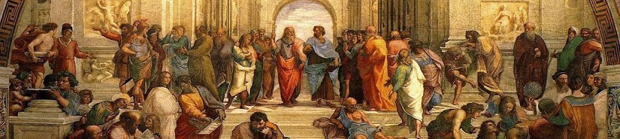
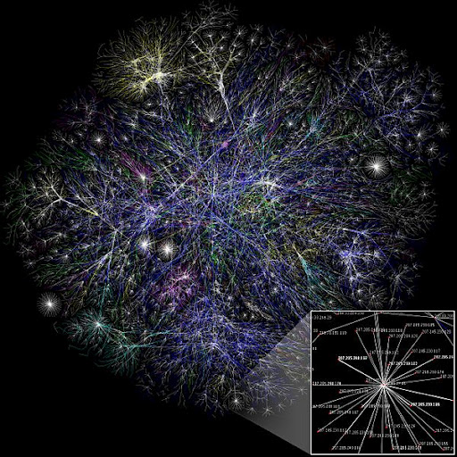

 -th mode
  is determined by the
  and the
  .
.

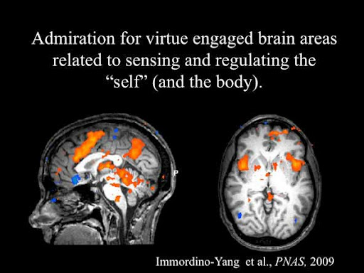

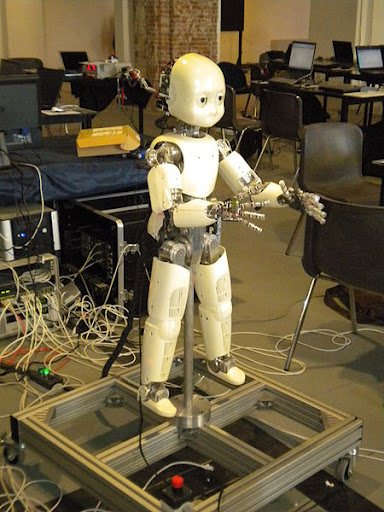


 or
or  . Limiting-recursion, by contrast, can compute any predicate or function in the corresponding
  . Gold further showed that limiting partial recursion would allow the computation of precisely the
  predicates.
 )
)
![\Delta^0_1[f]](https://i0.wp.com/upload.wikimedia.org/wikipedia/en/math/d/d/9/dd9474960ab9e8e906912bdf3e92b108.png)


 are r.e.
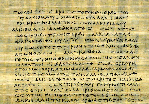
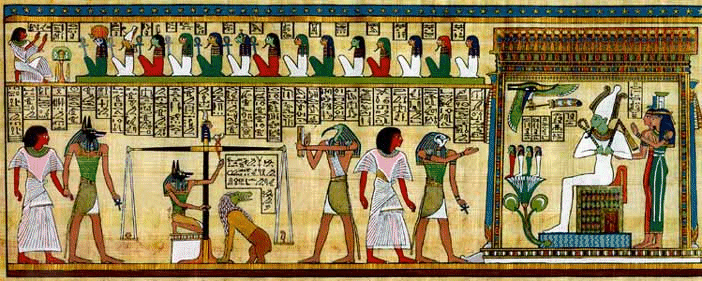
